Select the "Begin" button to start.
Capital Budgeting Decision
Introduction
This activity begins with a demonstration about how net present value is calculated based on a scenario of a company considering the financial impact of purchasing a new machine to manufacture a product. You will be asked to make the last calculation to determine the net present value and then decide the best course of action. A final activity will allow you to manipulate various factors impacting present values associated with a variety of business related investment options.
Question
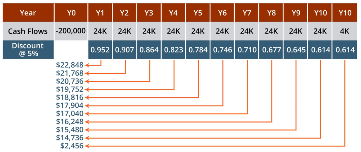
Considering the values provided in the table, what is the net present value (NPV) of the new machine?
No, that is not the correct answer. Try Again.
Yes, -$12,216 is the correct answer.
Hint: Make sure to sum up all the present values for each year plus the PV of the salvage amount. Remember to factor in the PV of the machine based on its initial cost of $200,000. The purchase price of the machine is a cash outflow, so give it a negative value.
Hint: Adding $187,784 to a negative $200,000, will give you the correct answer.
Question
Should the company purchase the new machine or not?
Correct! The NPV is -$12,216. The general rule is that if a project’s NPV is positive, then the project is at least minimally acceptable because another use of those funds is not expected to generate a better return. If the project’s NPV is negative, then the project is not minimally acceptable. Since the NPV is negative, we should not invest.
Incorrect. The NPV is -$12,216. Think about the direction of the NPV. This is not the most appropriate decision.
Shortcut to Determining Net Present Value
We have gone through an exercise using a graphical approach to depict the concept of net present value while utilizing a formula to calculate the present value of each cash flow. However, there are present value factor tables that can be used to arrive at a net present value and, thus, do not require the calculation of each present value factor to determine individual cash flow present values. These tables will be provided to you on quiz and test questions requiring the use of present value factors.
The following is a section taken from one such table displaying the present value of one dollar received at the end of each period at an interest rate of 5 percent and corresponds to the values previously calculated. Adding up the discount factors for each period at a discount rate of 5 percent will give 7.72. Multiplying 7.72 to $24,000 gives $185,328. Adding this to the product of $4000 times 0.614, which is $2,456, results in a present value of $187,784. This is the same value derived from the formula used in this exercise.
|
Periods |
3% |
4% |
5% |
6% |
7% |
8% |
|
1 |
.971 |
.962 |
.952 |
.943 |
.935 |
.926 |
|
2 |
.943 |
.925 |
.907 |
.890 |
.873 |
.857 |
|
3 |
.915 |
.889 |
.864 |
.840 |
.816 |
.794 |
|
4 |
.888 |
.855 |
.823 |
.792 |
.763 |
.735 |
|
5 |
.863 |
.822 |
.784 |
.747 |
.713 |
.681 |
|
6 |
.837 |
.790 |
.746 |
.705 |
.666 |
.630 |
|
7 |
.813 |
.760 |
.711 |
.665 |
.623 |
.583 |
|
8 |
.789 |
.731 |
.677 |
.627 |
.582 |
.540 |
|
9 |
.766 |
.703 |
.645 |
.592 |
.544 |
.500 |
|
10 |
.744 |
.676 |
.614 |
.558 |
.508 |
.463 |
Similarly, present values of streams of equal cash flows can be computed by referring to a present value of an annuity table. The present value factor highlighted below represents the present value factor used to discount a stream of dollars received at the end of each of 10 periods at an interest rate of 5 percent. Referring to the table, this value is 7.722, the same as calculated using the formula and derived from the present value factor table. This is a quicker approach to computing the present value of a stream of equal cash flows that all occur over equal intervals of time.
|
Periods |
3% |
4% |
5% |
6% |
7% |
8% |
|
1 |
.971 |
.962 |
.952 |
.943 |
.935 |
.926 |
|
2 |
1.913 |
1.886 |
1.859 |
1.833 |
1.808 |
1.783 |
|
3 |
2.829 |
2.775 |
2.723 |
2.673 |
2.624 |
2.577 |
|
4 |
3.717 |
3.630 |
3.546 |
3.465 |
3.387 |
3.312 |
|
5 |
4.580 |
4.452 |
4.329 |
4.212 |
4.100 |
3.993 |
|
6 |
5.417 |
5.242 |
5.076 |
4.917 |
4.767 |
4.623 |
|
7 |
6.230 |
6.002 |
5.786 |
5.582 |
5.389 |
5.206 |
|
8 |
7.020 |
6.733 |
6.463 |
6.210 |
5.971 |
5.747 |
|
9 |
7.786 |
7.435 |
7.108 |
6.802 |
6.515 |
6.247 |
|
10 |
8.530 |
8.111 |
7.722 |
7.360 |
7.024 |
6.710 |
Experiment with computing the net present value of a similar project. Try changing the number of periods for the life of the asset, the opportunity cost of capital interest rate, the annual cash savings amount, and the salvage value. Investigate how changes in each of these variables impacts the net present value.
|
Periods |
3% |
4% |
5% |
6% |
7% |
8% |
|
1 |
.971 |
.962 |
.952 |
.943 |
.935 |
.926 |
|
2 |
.943 |
.925 |
.907 |
.890 |
.873 |
.857 |
|
3 |
.915 |
.889 |
.864 |
.840 |
.816 |
.794 |
|
4 |
.888 |
.855 |
.823 |
.792 |
.763 |
.735 |
|
5 |
.863 |
.822 |
.784 |
.747 |
.713 |
.681 |
|
6 |
.837 |
.790 |
.746 |
.705 |
.666 |
.630 |
|
7 |
.813 |
.760 |
.711 |
.665 |
.623 |
.583 |
|
8 |
.789 |
.731 |
.677 |
.627 |
.582 |
.540 |
|
9 |
.766 |
.703 |
.645 |
.592 |
.544 |
.500 |
|
10 |
.744 |
.676 |
.614 |
.558 |
.508 |
.463 |
|
Periods |
3% |
4% |
5% |
6% |
7% |
8% |
|
1 |
.971 |
.962 |
.952 |
.943 |
.935 |
.926 |
|
2 |
1.913 |
1.886 |
1.859 |
1.833 |
1.808 |
1.783 |
|
3 |
2.829 |
2.775 |
2.723 |
2.673 |
2.624 |
2.577 |
|
4 |
3.717 |
3.630 |
3.546 |
3.465 |
3.387 |
3.312 |
|
5 |
4.580 |
4.452 |
4.329 |
4.212 |
4.100 |
3.993 |
|
6 |
5.417 |
5.242 |
5.076 |
4.917 |
4.767 |
4.623 |
|
7 |
6.230 |
6.002 |
5.786 |
5.582 |
5.389 |
5.206 |
|
8 |
7.020 |
6.733 |
6.463 |
6.210 |
5.971 |
5.747 |
|
9 |
7.786 |
7.435 |
7.108 |
6.802 |
6.515 |
6.247 |
|
10 |
8.530 |
8.111 |
7.722 |
7.360 |
7.024 |
6.710 |
Present values of the annuity stream:
Why did the net present values change the way that they did?